Measures

Default measures

Let’s quickly create a cube from a CSV file. You can see the value of your measures at the top level of the cube by calling cube.query():

import atoti as tt

session = tt.create_session()
store = session.read_csv("data/example.csv", keys=["ID"], store_name="First")
cube = session.create_cube(store, "FirstCube")
lvl = cube.levels
m = cube.measures
hier = cube.hierarchies
cube.query()

Welcome to atoti 0.4.0!

By using this community edition, you agree with the license available at https://www.atoti.io/eula.
Browse the official documentation at https://docs.atoti.io.
Join the community at https://www.atoti.io/register.

You can hide this message by setting the ATOTI_HIDE_EULA_MESSAGE environment variable to True.

	Price.MEAN	Price.SUM	Quantity.MEAN	Quantity.SUM	contributors.COUNT
0	428.0	4280.0	2270.0	22700.0	10

SUM and MEAN aggregations are automatically created for numeric columns.

Calling cube.query() will display the value of the measure at the top level. It’s also possible to specify levels to split the cube:

cube.query(m["Quantity.SUM"], levels=[lvl["Continent"], lvl["Country"]])

		Quantity.SUM
Continent	Country
Asia	China	6000.0
	India	3700.0
Europe	France	7500.0
	UK	5500.0

You can also filter on levels:

cube.query(
    m["Quantity.SUM"],
    levels=[lvl["Continent"], lvl["Country"]],
    condition=(lvl["Country"] == "France"),
)

		Quantity.SUM
Continent	Country
Europe	France	7500.0

Aggregation functions

The available aggregation functions are:

from inspect import getmembers, isfunction

[member[0] for member in getmembers(tt.agg) if isfunction(member[1])]

['_agg',
 '_count',
 '_vector',
 'array_quantile',
 'check_literal',
 'count_distinct',
 'doc',
 'long',
 'max',
 'max_member',
 'mean',
 'median',
 'min',
 'min_member',
 'prod',
 'quantile',
 'short',
 'single_value',
 'sqrt',
 'square_sum',
 'std',
 'stop',
 'sum',
 'var']

m["Quantity.MIN"] = tt.agg.min(store["Quantity"])
m["Quantity.MAX"] = tt.agg.max(store["Quantity"])
m["Quantity.LONG"] = tt.agg.long(store["Quantity"])
m["Quantity.SHORT"] = tt.agg.short(store["Quantity"])
cube.query(levels=[lvl["Country"]])

	Price.MEAN	Price.SUM	Quantity.LONG	Quantity.MAX	Quantity.MEAN	Quantity.MIN	Quantity.SHORT	Quantity.SUM	contributors.COUNT
Country
China	380.0	760.0	6000.0	4000.0	3000.0	2000.0	0.0	6000.0	2
France	450.0	1800.0	7500.0	3000.0	1875.0	1000.0	0.0	7500.0	4
India	380.0	760.0	3700.0	2200.0	1850.0	1500.0	0.0	3700.0	2
UK	480.0	960.0	5500.0	3000.0	2750.0	2500.0	0.0	5500.0	2

m["Quantity running sum"] = tt.agg.sum(
    m["Quantity.SUM"], scope=tt.scope.cumulative(lvl["ID"])
)
cube.query(m["Quantity running sum"], levels=[lvl["ID"]])

	Quantity running sum
ID
1	1000.0
2	3000.0
3	6000.0
4	7500.0
5	10500.0
6	13000.0
7	15000.0
8	19000.0
9	21200.0
10	22700.0

m["Distinct City"] = tt.agg.count_distinct(store["City"])

m["Quantile 95"] = tt.agg.quantile(store["Quantity"], 0.95)
m["Quantile 20"] = tt.agg.quantile(store["Quantity"], 0.20)
cube.query(m["Quantile 95"], m["Quantile 20"], levels=[lvl["Continent"]])

	Quantile 95	Quantile 20
Continent
Asia	3730.0	1800.0
Europe	3000.0	1500.0

Statistics aggregations

m["Quantity variance"] = tt.agg.var(store["Quantity"], mode="sample")
m["Quantity standard deviation"] = tt.agg.std(store["Quantity"], mode="sample")
cube.query(m["Quantity variance"], m["Quantity standard deviation"])

	Quantity variance	Quantity standard deviation
0	784555.555556	885.751407

MaxMember / MinMember

max_member and min_member search for the specified extremum of the given measure and return the member of the specified level for which the extremum is reached.

m["MinMember of Price.SUM"] = tt.agg.min_member(m["Price.SUM"], lvl["City"])
m["MaxMember of Price.SUM"] = tt.agg.max_member(m["Price.SUM"], lvl["City"])

cube.query(m["MinMember of Price.SUM"], m["MaxMember of Price.SUM"])

	MinMember of Price.SUM	MaxMember of Price.SUM
0	HongKong	London

No matter which level you execute the query on, the argmin is always performed at the level specified when defining the measure

cube.query(
    m["MinMember of Price.SUM"],
    m["MaxMember of Price.SUM"],
    levels=[lvl["Continent"], lvl["Country"]],
)

		MinMember of Price.SUM	MaxMember of Price.SUM
Continent	Country
Asia	China	HongKong	Beijing
	India	Dehli	Mumbai
Europe	France	Lyon	Paris
	UK	London	London

Delete a measure

Any measure can be removed from the cube using del

"Quantity running sum" in m

True

del m["Quantity running sum"]
"Quantity running sum" in m

False

Different aggregations per level

It’s possible to aggregate a column differently depending on whether we are above or below a certain level.

For example, you can sum a quantity for each country and then take the average over all the countries:

m["Average per country"] = tt.agg.mean(
    m["Quantity.SUM"], scope=tt.scope.origin(lvl["Country"])
)
cube.query(m["Average per country"], levels=[lvl["Country"]])

	Average per country
Country
China	6000.0
France	7500.0
India	3700.0
UK	5500.0

cube.query(m["Average per country"])

	Average per country
0	5675.0

Calculated measures

Measures can be combined together to build more complex measures:

m["Turnover"] = tt.agg.sum(m["Quantity.SUM"] * store["Price"])
cube.query(levels=[lvl["Country"]])

	Average per country	Distinct City	MaxMember of Price.SUM	MinMember of Price.SUM	Price.MEAN	Price.SUM	Quantile 20	Quantile 95	Quantity standard deviation	Quantity variance	Quantity.LONG	Quantity.MAX	Quantity.MEAN	Quantity.MIN	Quantity.SHORT	Quantity.SUM	Turnover	contributors.COUNT
Country
China	6000.0	2	Beijing	HongKong	380.0	760.0	2400.0	3900.0	1414.213562	2.000000e+06	6000.0	4000.0	3000.0	2000.0	0.0	6000.0	2220000.0	2
France	7500.0	3	Paris	Lyon	450.0	1800.0	1300.0	2850.0	853.912564	7.291667e+05	7500.0	3000.0	1875.0	1000.0	0.0	7500.0	3280000.0	4
India	3700.0	2	Mumbai	Dehli	380.0	760.0	1640.0	2165.0	494.974747	2.450000e+05	3700.0	2200.0	1850.0	1500.0	0.0	3700.0	1392000.0	2
UK	5500.0	1	London	London	480.0	960.0	2600.0	2975.0	353.553391	1.250000e+05	5500.0	3000.0	2750.0	2500.0	0.0	5500.0	2630000.0	2

Multidimensional Functions

Parent Value

# Create multi-level hierarchy :
lvl = cube.levels
cube.hierarchies["Geography"] = {
    "continent": lvl["Continent"],
    "country": lvl["Country"],
    "city": lvl["City"],
}

help(tt.parent_value)

Help on function parent_value in module atoti._functions.multidimensional:

parent_value(measure: 'Union[Measure, str]', on: 'Hierarchy', *, apply_filters: 'bool' = False, degree: 'int' = 1, total_value: 'Optional[MeasureLike]' = None) -> 'Measure'
    Return a measure equal to the passed measure at the parent member on the given hierarchy.

    Example:
        Measure definitions::

            m1 = parent_value(Quantity.SUM, Date)
            m2 = parent_value(Quantity.SUM, Date, degree=3)
            m3 = parent_value(Quantity.SUM, Date, degree=3, total_value=Quantity.SUM))
            m4 = parent_value(Quantity.SUM, Date, degree=3, total_value=Other.SUM))

        Considering a non slicing hierarchy ``Date`` with three levels ``Years``, ``Month`` and ``Day``:

        +------------+-------+-----+--------------+-----------+-------+-------+-------+-------+
        | Year       | Month | Day | Quantity.SUM | Other.SUM | m1    | m2    | m3    | m4    |
        +============+=======+=====+==============+===========+=======+=======+=======+=======+
        | 2019       |       |     | 75           | 1000      | 110   | null  | 110   | 1500  |
        +------------+-------+-----+--------------+-----------+-------+-------+-------+-------+
        |            |  7    |     | 35           | 750       | 75    | null  | 110   | 1500  |
        +------------+-------+-----+--------------+-----------+-------+-------+-------+-------+
        |            |       | 1   | 15           | 245       | 35    | 110   | 110   | 110   |
        +------------+-------+-----+--------------+-----------+-------+-------+-------+-------+
        |            |       | 2   | 20           | 505       | 35    | 110   | 110   | 110   |
        +------------+-------+-----+--------------+-----------+-------+-------+-------+-------+
        |            |  6    |     | 40           | 250       | 75    | null  | 110   | 1500  |
        +------------+-------+-----+--------------+-----------+-------+-------+-------+-------+
        |            |       | 1   | 25           | 115       | 40    | 110   | 110   | 110   |
        +------------+-------+-----+--------------+-----------+-------+-------+-------+-------+
        |            |       | 2   | 15           | 135       | 40    | 110   | 110   | 110   |
        +------------+-------+-----+--------------+-----------+-------+-------+-------+-------+
        | 2018       |       |     | 35           | 500       | 110   | null  | 110   | 1500  |
        +------------+-------+-----+--------------+-----------+-------+-------+-------+-------+
        |            |  7    |     | 15           | 200       | 35    | null  | 110   | 1500  |
        +------------+-------+-----+--------------+-----------+-------+-------+-------+-------+
        |            |       | 1   | 5            | 55        | 15    | 110   | 110   | 110   |
        +------------+-------+-----+--------------+-----------+-------+-------+-------+-------+
        |            |       | 2   | 10           | 145       | 15    | 110   | 110   | 110   |
        +------------+-------+-----+--------------+-----------+-------+-------+-------+-------+
        |            |  6    |     | 20           | 300       | 35    | null  | 110   | 1500  |
        +------------+-------+-----+--------------+-----------+-------+-------+-------+-------+
        |            |       | 1   | 15           | 145       | 20    | 110   | 110   | 110   |
        +------------+-------+-----+--------------+-----------+-------+-------+-------+-------+
        |            |       | 2   | 5            | 155       | 20    | 110   | 110   | 110   |
        +------------+-------+-----+--------------+-----------+-------+-------+-------+-------+

        Considering a slicing hierarchy ``Date`` with three levels ``Years``, ``Month`` and ``Day``:

        +------------+-------+-----+--------------+-----------+-------+-------+-------+-------+
        | Year       | Month | Day | Quantity.SUM | Other.SUM | m1    | m2    | m3    | m4    |
        +============+=======+=====+==============+===========+=======+=======+=======+=======+
        | 2019       |       |     | 75           | 1000      | 75    | null  | 75    | 1000  |
        +------------+-------+-----+--------------+-----------+-------+-------+-------+-------+
        |            |  7    |     | 35           | 750       | 75    | null  | 75    | 1000  |
        +------------+-------+-----+--------------+-----------+-------+-------+-------+-------+
        |            |       | 1   | 15           | 245       | 35    | 75    | 75    | 75    |
        +------------+-------+-----+--------------+-----------+-------+-------+-------+-------+
        |            |       | 2   | 20           | 505       | 35    | 75    | 75    | 75    |
        +------------+-------+-----+--------------+-----------+-------+-------+-------+-------+
        |            |  6    |     | 40           | 250       | 75    | null  | 75    | 1000  |
        +------------+-------+-----+--------------+-----------+-------+-------+-------+-------+
        |            |       | 1   | 25           | 115       | 40    | 75    | 75    | 75    |
        +------------+-------+-----+--------------+-----------+-------+-------+-------+-------+
        |            |       | 2   | 15           | 135       | 40    | 75    | 75    | 75    |
        +------------+-------+-----+--------------+-----------+-------+-------+-------+-------+
        | 2018       |       |     | 35           | 500       | 35    | null  | 35    | 500   |
        +------------+-------+-----+--------------+-----------+-------+-------+-------+-------+
        |            |  7    |     | 15           | 200       | 35    | null  | 35    | 500   |
        +------------+-------+-----+--------------+-----------+-------+-------+-------+-------+
        |            |       | 1   | 5            | 55        | 15    | 35    | 35    | 35    |
        +------------+-------+-----+--------------+-----------+-------+-------+-------+-------+
        |            |       | 2   | 10           | 145       | 15    | 35    | 35    | 35    |
        +------------+-------+-----+--------------+-----------+-------+-------+-------+-------+
        |            |  6    |     | 20           | 300       | 35    | null  | 35    | 500   |
        +------------+-------+-----+--------------+-----------+-------+-------+-------+-------+
        |            |       | 1   | 15           | 145       | 20    | 35    | 35    | 35    |
        +------------+-------+-----+--------------+-----------+-------+-------+-------+-------+
        |            |       | 2   | 5            | 155       | 20    | 35    | 35    | 35    |
        +------------+-------+-----+--------------+-----------+-------+-------+-------+-------+

    Args:
        measure: The measure to take the parent value of.
        on: The hierarchy to drill up to take the parent value.
        apply_filters: Whether to apply the query filters when computing the
            value at the parent member.
        degree: The number of levels to go up to take the value on. A value
            of ``1`` as parent_degree will do a one step drill up in the hierarchy.
        total_value: The value to take when the drill up went above the top level of the hierarchy.

m["Parent quantity"] = tt.parent_value(m["Quantity.SUM"], on=hier["Geography"])

We can check that the value on countries is equal to the Quantity.SUM on their continent :

cube.query(m["Parent quantity"], levels=[lvl["continent"], lvl["country"]])

		Parent quantity
continent	country
Asia	China	9700.0
	India	9700.0
Europe	France	13000.0
	UK	13000.0

cube.query(m["Quantity.SUM"], levels=[lvl["continent"]])

	Quantity.SUM
continent
Asia	9700.0
Europe	13000.0

Aggregate siblings

Siblings are all the children of the same member. For instance France and UK are children of Europe so France and UK are siblings.

m["Sum siblings"] = tt.agg.sum(
    m["Quantity.SUM"], scope=tt.scope.siblings(hier["Geography"])
)
cube.query(m["Sum siblings"], levels=[lvl["country"], lvl["city"]])

			Sum siblings
continent	country	city
Asia	China	Beijing	6000.0
		HongKong	6000.0
	India	Dehli	3700.0
		Mumbai	3700.0
Europe	France	Bordeaux	7500.0
		Lyon	7500.0
		Paris	7500.0
	UK	London	5500.0

m["Average siblings"] = tt.agg.mean(
    m["Quantity.SUM"], scope=tt.scope.siblings(hier["Geography"])
)
cube.query(m["Average siblings"], levels=[lvl["country"], lvl["city"]])

			Average siblings
continent	country	city
Asia	China	Beijing	3000.0
		HongKong	3000.0
	India	Dehli	1850.0
		Mumbai	1850.0
Europe	France	Bordeaux	2500.0
		Lyon	2500.0
		Paris	2500.0
	UK	London	5500.0

Shift

shift allows to get the value of previous or next members on a level

m["next quantity"] = tt.shift(m["Quantity.SUM"], on=lvl["Date"], offset=1)
cube.query(m["next quantity"], levels=[lvl["Date"]])

	next quantity
Date
2018-01-01	8000.0
2019-01-01	4000.0
2019-01-02	7000.0

cube.query(m["Quantity.SUM"], levels=[lvl["Date"]])

	Quantity.SUM
Date
2018-01-01	3700.0
2019-01-01	8000.0
2019-01-02	4000.0
2019-01-05	7000.0

Filter

filter allows you to only express the measure where certain conditions are met.

You can only use conditions on levels with filter. If you want to use conditions involving measures you should use where.

You can combine conditions with the & bitwise operator.

m["Filtered Quantity.SUM"] = tt.filter(
    m["Quantity.SUM"], (lvl["City"] == "Paris") & (lvl["Color"] == "red")
)
cube.query(
    m["Quantity.SUM"], m["Filtered Quantity.SUM"], levels=[lvl["Country"], lvl["Color"]]
)

		Quantity.SUM	Filtered Quantity.SUM
Country	Color
China	blue	2000.0	NaN
	green	4000.0	NaN
France	blue	4500.0	NaN
	red	3000.0	1000.0
India	blue	1500.0	NaN
	red	2200.0	NaN
UK	green	3000.0	NaN
	red	2500.0	NaN

Where

where defines an if-then-else measure whose value depends on certain conditions. It is similar to numpy’s where function.

# Label large amounts
m["Large quantities"] = tt.where(m["Quantity.SUM"] >= 3000, "large", "small")

# Double up UK's quantities
m["Double UK"] = tt.where(
    lvl["Country"] == "UK", 2 * m["Quantity.SUM"], m["Quantity.SUM"]
)

cube.query(
    m["Quantity.SUM"],
    m["Large quantities"],
    m["Double UK"],
    levels=[lvl["Country"], lvl["Color"]],
)

		Quantity.SUM	Large quantities	Double UK
Country	Color
China	blue	2000.0	small	2000.0
	green	4000.0	large	4000.0
France	blue	4500.0	large	4500.0
	red	3000.0	large	3000.0
India	blue	1500.0	small	1500.0
	red	2200.0	small	2200.0
UK	green	3000.0	large	6000.0
	red	2500.0	small	5000.0

At

at takes the value of the given measure shifted on one of the level to the given value.

The value can be a literal value or the value of another level

m["Blue Quantity"] = tt.at(m["Quantity.SUM"], {lvl["Color"]: "blue"})
cube.query(m["Quantity.SUM"], m["Blue Quantity"], levels=[lvl["Color"]])

	Quantity.SUM	Blue Quantity
Color
blue	8000.0	8000.0
green	7000.0	8000.0
red	7700.0	8000.0

The measure is null if the level is not expressed

cube.query(m["Quantity.SUM"], m["Blue Quantity"])

	Quantity.SUM	Blue Quantity
0	22700.0	None

In a multilevel hierarchy, only the shifted level is changed. For instance if we shift the country to “France”, [Europe, UK] is shifted to [Europe,France] and [Asia,China] is shifted to [Asia,France] which does not exist.

m["France Quantity Fail"] = tt.at(m["Quantity.SUM"], {lvl["country"]: "France"})
cube.query(
    m["Quantity.SUM"],
    m["France Quantity Fail"],
    levels=[lvl["continent"], lvl["country"]],
)

		Quantity.SUM	France Quantity Fail
continent	country
Asia	China	6000.0	NaN
	India	3700.0	NaN
Europe	France	7500.0	7500.0
	UK	5500.0	7500.0

The expected value can be obtained by shifting both levels to the requested values as follow.

m["France Quantity"] = tt.at(
    m["Quantity.SUM"], {lvl["country"]: "France", lvl["continent"]: "Europe"}
)
cube.query(
    m["Quantity.SUM"], m["France Quantity"], levels=[lvl["continent"], lvl["country"]]
)

		Quantity.SUM	France Quantity
continent	country
Asia	China	6000.0	7500.0
	India	3700.0	7500.0
Europe	France	7500.0	7500.0
	UK	5500.0	7500.0

Other Functions

Mathematical functions

round, floor, and ceil: closest, lower, and upper rounding of double values

m["round"] = tt.round(m["Quantity.SUM"] / 1000) * 1000
m["floor"] = tt.floor(m["Quantity.SUM"] / 1000) * 1000
m["ceil"] = tt.ceil(m["Quantity.SUM"] / 1000) * 1000
cube.query(
    m["Quantity.SUM"], m["floor"], m["ceil"], m["round"], levels=[lvl["Country"]]
)

	Quantity.SUM	floor	ceil	round
Country
China	6000.0	6000	6000	6000
France	7500.0	7000	8000	8000
India	3700.0	3000	4000	4000
UK	5500.0	5000	6000	6000

exp: Exponential is Euler’s number e raised to the power of a double value.

m["Zero"] = 0.0
m["One"] = tt.exp(m["Zero"])

log: the natural (base e) logarithm

m["Log Quantity"] = tt.log(m["Quantity.SUM"])
cube.query(m["Log Quantity"], levels=[lvl["Country"]])

	Log Quantity
Country
China	8.699515
France	8.922658
India	8.216088
UK	8.612503

log10: the base 10 logarithm

m["Log10 Quantity"] = tt.log10(m["Quantity.SUM"])
cube.query(m["Log10 Quantity"], levels=[lvl["Country"]])

	Log10 Quantity
Country
China	3.778151
France	3.875061
India	3.568202
UK	3.740363

abs: the absolute value of a given measure

m["Negative"] = -1 * m["Quantity.SUM"]
m["abs"] = tt.abs(m["Negative"])
cube.query(m["abs"])

	abs
0	22700.0

sin: the sinus value of a given measure

m["Sinus Quantity"] = tt.sin(m["Quantity.SUM"])
cube.query(m["Sinus Quantity"], levels=[lvl["Country"]])

	Sinus Quantity
Country
China	-0.427720
France	-0.851236
India	-0.714666
UK	0.800864

cos: the cosinus value of a given measure

m["Cosinus Quantity"] = tt.cos(m["Quantity.SUM"])
cube.query(m["Cosinus Quantity"], levels=[lvl["Country"]])

	Cosinus Quantity
Country
China	0.903912
France	-0.524783
India	0.699466
UK	-0.598846

tan: the tangent value of a given measure

m["Tangent Quantity"] = tt.tan(m["Quantity.SUM"])
cube.query(m["Tangent Quantity"], levels=[lvl["Country"]])

	Tangent Quantity
Country
China	-0.473187
France	1.622071
India	-1.021730
UK	-1.337344

pow: the calculated power value of a given measure

m["Power int Quantity"] = m["Quantity.SUM"] ** 2
cube.query(m["Power int Quantity"], levels=[lvl["Country"]])

	Power int Quantity
Country
China	36000000.0
France	56250000.0
India	13690000.0
UK	30250000.0

m["Power float Quantity"] = m["Quantity.SUM"] ** 0.5
cube.query(m["Power float Quantity"], levels=[lvl["Country"]])

	Power float Quantity
Country
China	77.459667
France	86.602540
India	60.827625
UK	74.161985

m["Power measure Quantity"] = m["Quantity.SUM"] ** m["Quantity.SUM"]
cube.query(m["Power measure Quantity"], levels=[lvl["Country"]])

	Power measure Quantity
Country
China	Infinity
France	Infinity
India	Infinity
UK	Infinity

m["Power neg Quantity"] = m["Quantity.SUM"] ** -3
cube.query(m["Power neg Quantity"], levels=[lvl["Country"]])

	Power neg Quantity
Country
China	4.629630e-12
France	2.370370e-12
India	1.974217e-11
UK	6.010518e-12

sqrt: the square root value of a given measure

m["Sqrt Quantity"] = tt.sqrt(m["Quantity.SUM"])
cube.query(m["Sqrt Quantity"], levels=[lvl["Country"]])

	Sqrt Quantity
Country
China	77.459667
France	86.602540
India	60.827625
UK	74.161985

Time functions

date_diff is the number of days between 2 dates:

from datetime import datetime

lvl = cube.levels
m["Days from today"] = tt.date_diff(datetime.now().date(), lvl["Date"])
cube.query(m["Days from today"], levels=[lvl["Date"]])

	Days from today
Date
2018-01-01	-875
2019-01-01	-510
2019-01-02	-509
2019-01-05	-506

Measure Folder

Measures can be put into folders to group them in the UI.

for name in [
    "Quantity.SUM",
    "Quantity.MEAN",
    "Quantity.LONG",
    "Quantity.MAX",
    "Quantity.MIN",
    "Quantity.SHORT",
]:
    m[name].folder = "Quantity"

m["Quantity.SUM"].folder

'Quantity'

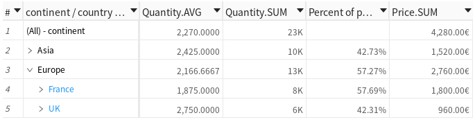
Measure formatter

Measures have formatters describing how to represent them as strings. These formatters can be modified in Python or directly in the UI. Here are a few examples of what is possible, more documentation on how to write an MDX formatter can be found on docs.microsoft.com.

# Convert to thousands
m["Quantity.SUM"].formatter = "DOUBLE[#,###,K]"

# Add a unit
m["Price.SUM"].formatter = "DOUBLE[#,###.00€]"

# Add more decimal figures
m["Quantity.MEAN"].formatter = "DOUBLE[#,###.0000]"

# Display as percent
m["Percent of parent"] = m["Quantity.SUM"] / m["Parent quantity"]
m["Percent of parent"].formatter = "DOUBLE[#,###.00%]"